Auditing Bias in Automated Decision-Making Systems
Author
Lukka Wolff
Published
March 12, 2025
Abstract
This project audits bias in automated decision-making systems by analyzing employment predictions from the 2018 American Community Survey (ACS) data for Georgia. A Random Forest Classifier was trained to predict employment status based on demographic features such as age, education, sex, disability, and nativity, while examining racial bias specifically between White and Black/African American individuals. The audit revealed approximately balanced accuracy, positive predictive values, and error rates across these racial groups, though slight discrepancies exist. Despite good numerical fairness, we must still consider ethical considerations regarding consent, data recency, and the ethical deployment of such models in different decision-making contexts.
Data and Feature Selection
We are using the folkables package to access data from the 2018 American Community Survey’s Public Use Microdata Sample (PUMS) for the state of Georgia.
from folktables import ACSDataSource, ACSEmployment, BasicProblem, adult_filterimport numpy as npSTATE ="GA"data_source = ACSDataSource(survey_year='2018', horizon='1-Year', survey='person')acs_data = data_source.get_data(states=[STATE], download=True)acs_data.head()
RT
SERIALNO
DIVISION
SPORDER
PUMA
REGION
ST
ADJINC
PWGTP
AGEP
...
PWGTP71
PWGTP72
PWGTP73
PWGTP74
PWGTP75
PWGTP76
PWGTP77
PWGTP78
PWGTP79
PWGTP80
0
P
2018GQ0000025
5
1
3700
3
13
1013097
68
51
...
124
69
65
63
117
66
14
68
114
121
1
P
2018GQ0000035
5
1
1900
3
13
1013097
69
56
...
69
69
7
5
119
74
78
72
127
6
2
P
2018GQ0000043
5
1
4000
3
13
1013097
89
23
...
166
88
13
13
15
91
163
13
89
98
3
P
2018GQ0000061
5
1
500
3
13
1013097
10
43
...
19
20
3
9
20
3
3
10
10
10
4
P
2018GQ0000076
5
1
4300
3
13
1013097
11
20
...
13
2
14
2
1
2
2
13
14
12
5 rows × 286 columns
This data set contains a large amount of features for each individual, so we are going to narrow it down to only those that we may use to train our model.
ESR is employment status (1 if employed, 0 if not)
RAC1P is race (1 for White Alone, 2 for Black/African American Alone, 3 and above for other self-identified racial groups)
SEX is binary sex (1 for male, 2 for female)
Now we select for the features we want to use and we will be able to constuct a BasicProblem that expresses our desire to use these features to predict employment status ESR, using RAC1P as the group label.
features_to_use = [f for f in possible_features if f notin ["ESR", "RAC1P"]]
The two largest racial groups are 1 White Alone with 53302 individuals making up 66% of the data, and 2 Black/African American Alone with 20239 individuals making up 25% of the data.
~46% of White Alone individuals are employed and ~42% of Black/African American Alone individuals are employed.
import seaborn as snsimport matplotlib.pyplot as pltsns.set_theme(style="whitegrid")
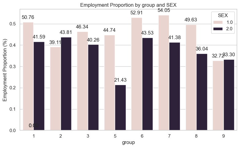
def plot_intersection(df, col1='group', col2='sex'): prop_df = df.groupby([col1, col2])['label'].mean().reset_index() plt.figure(figsize=(8, 5)) ax = sns.barplot(x=col1, y='label', hue=col2, data=prop_df) plt.title(f'Employment Proportion by {col1} and {col2}') plt.xlabel(col1) plt.ylabel(f'Employment Proportion (%)')for p in ax.patches: ax.annotate(f'{p.get_height()*100:.2f}', (p.get_x() + p.get_width() /2., p.get_height()), ha ='center', va ='bottom', xytext = (0, 5), textcoords ='offset points') plt.tight_layout() plt.show()group_sex = plot_intersection(df, 'group', 'SEX')
For many groups, the percentage of men who are employed is higher than that of women. One notable group where this is not the case is 2 Black/African American where the percentage of employed women is ~44% against ~39% for men.
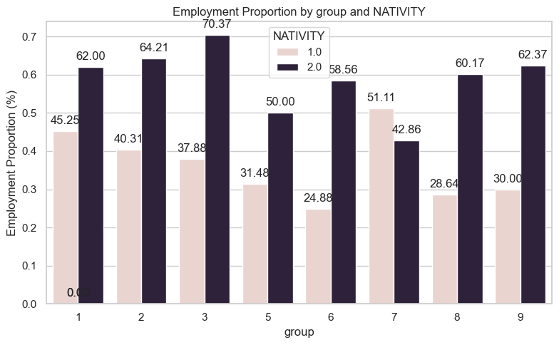
NATIVITY indicates a persons place of birth. 1 being Native born and 2 being Foreign born.
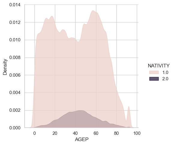
Interestingly, across the board we see that the percentage of foreign born individuals who are employed is much higher than the proportion of native born individuals. However, as seen in the plot below, this may be attributed to the fact that few foreign born individuals on the extremities of the age, reducing the influence of youth and seniority as factors in employment proportion.
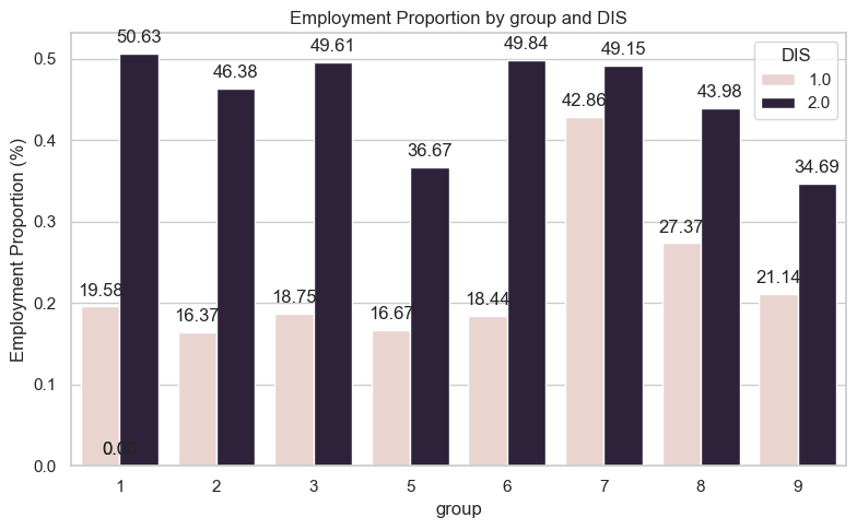
DIS represents an individuals disability status. 1 with disability, and 2 without a disability.
group_dis = plot_intersection(df, 'group', 'DIS')
Across the board we see that people without disability are employed at a much higher proportion than people with disabilities.
Supplementary plots that I thought were interesting.
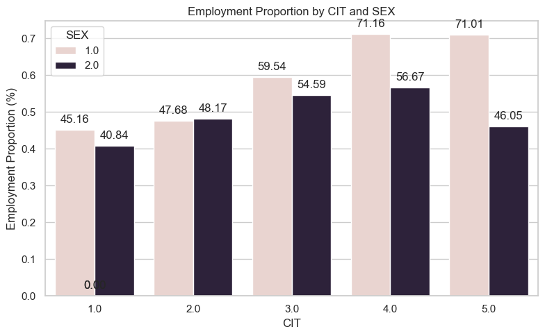
cit_sex = plot_intersection(df, 'CIT', 'SEX')
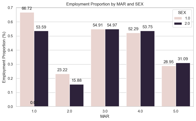
mar_sex = plot_intersection(df, 'MAR', 'SEX')
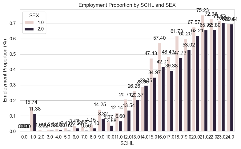
schl_sex = plot_intersection(df, 'SCHL', 'SEX')
Model Training
We are now ready to create a model and train it on our training data. We will first scale our data, then we will employ a Random Forest Classifier. This approach uses an array of decision trees on various sub-samples of the data and aggregates their results. Learn more here.
Above, we tuned our model complexity using the max_depth parameter of the RandomForestClassifier. This controls how deep each tree in our forest can get which impacts how general our model is with regards to things like overfitting. We examined values ranging from 5 to 20 for the max depth and found the highest cross validated accuracy when max_depth=16.
In a Jupyter environment, please rerun this cell to show the HTML representation or trust the notebook. On GitHub, the HTML representation is unable to render, please try loading this page with nbviewer.org.
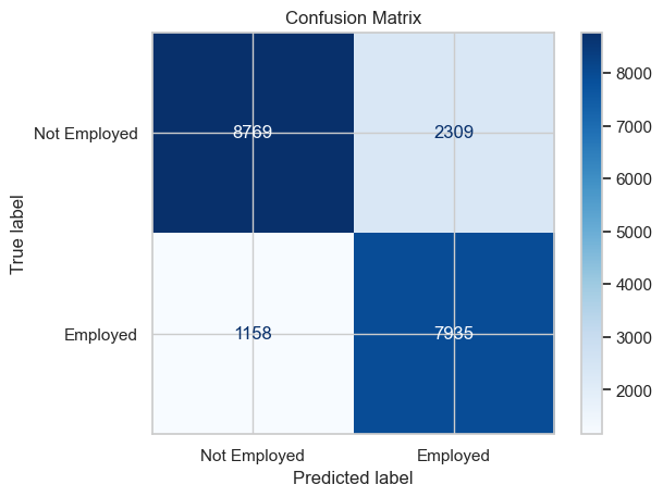
Our model has an overall accuracy of 82.81% on the testing data suite. Not too shabby!
We will now address the positive predictive value (PPV) of our model (we wont evaluate true sufficiency right now as we are skipping NPV). Given that the prediction is positive (y_hat = 1), how likely is it that the prediction is accurate (y_test = 1)? In other words, if we predict someone to be employed, how likely is it that they are actually employed?
We can approximate this value with the following code:
Our model incorrectly classified people as employed when they were in fact unemployed 20.84% of the time.
By-Group Measures
Now, lets explore how our model treats people in their respective groups. We are going to focus primarily on the possible discrepancies between individuals in 1 White Alone and 2 Black/African American Alone groups.
wa = (y_hat == y_test)[group_test ==1].mean()aa = (y_hat == y_test)[group_test ==2].mean()print(f"White Alone Accuracy: {wa*100:.2f}%\nBlack/African American Alone Accuracy: {aa*100:.2f}%")
White Alone Accuracy: 82.40%
Black/African American Alone Accuracy: 83.17%
Our model has pretty comparable accuracy scores for both groups, only slightly lower for White Alone individuals.
FPR for White Alone: 21.33%
FPR for Black/African American Alone: 19.64%
There is some slight discrepancy here as persons in the White Alone group is more often mistaken for having a job than persons in the Black/African American Alone group.
Bias Measures
In terms of accuracy, our model seems to be performing well. Let’s take a deeper look at how our model might be biased or unfair by examining calibration, error rate balance, and statistical parity.
Our model can be considered well-calibrated or sufficient if it reflects equal likelihood of employment irrespective of the individuals’ group membership. That is, free from predictive bias, this our PPV for both groups should be the same. Looking back to our calculation of these scores, we saw that they were about equal. PPV for White Alone: 77.96% and PPV for Black/African American Alone: 75.84%. Thus, we can say our model is well-calibrated.
Our model can only satisfy approximate error rate balance given that the true positive rate (TPR) and false positive rates (FPR) be equal on the two groups.
We can see that both groups have an approximately equal TPR and FPRs. Thus our model satisfies approximate error rate balance.
Our model satisfies statistical parity if the proportion of individuals classified as employed is the same for each group.
prop_wa = (y_hat ==1)[group_test ==1].mean()prop_aa = (y_hat ==1)[group_test ==2].mean()print(f"Proportion of White Alone Predicted to be Employed: {prop_wa*100:.2f}%")print(f"Proportion of Black/African American Alone Predicted to be Employed: {prop_aa*100:.2f}%")
Proportion of White Alone Predicted to be Employed: 51.74%
Proportion of Black/African American Alone Predicted to be Employed: 47.61%
We can observe some differences in these two scores, a higher proportion of White Alone persons are predicted to be employed than Black/African American Alone persons. The difference remains small as the rated are within 5% of one another… as we don’t have a set threshold we cant know if the difference is significant, ergo we cant say that we do or do not satisfy statistical parity.
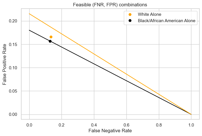
Feasible FNR and FPRs
p_wa = ((y_test ==1) & (y_hat ==1))[group_test ==1].mean()p_aa = ((y_test ==1) & (y_hat ==1))[group_test ==2].mean()print(f"Prevalence of White Alone: {p_wa*100:.2f}%")print(f"Prevalence of Black/African American Alone: {p_aa*100:.2f}%")
Prevalence of White Alone: 40.34%
Prevalence of Black/African American Alone: 36.11%
The proportion of true positive values is higher with in the White Alone group.
Our current model appears to be working quite well for both groups as we can see their (FNR, FPR) points are not far separated. However, if we did want to equalize our false positive rates (classify someone as employed when they are not), this would necessitate an increase in the false negative rates for White Alone to around 0.22 from its current around 0.12. This would inevitably lead to a drop in accuracy. Contextually, this would mean classifying more White Alone persons who are actually employed as unemployed to match FPR.
Nonetheless, our model performs close to even for both groups.
Conclusion
There are many applications for a model of this sort. Making predictions on who is or isn’t employed would benefit many companies that operate on credit or lending. Knowing who is employed would help determine whether it would be wise to approve a higher credit limit, approve a mortgage application, or let someone lease a car. This is the case because employment can be widely used aa feature or indicator of someones ability to pay back their debts and the interest included therein. If you determine that better, your company can be more profitable. This could also be useful for marketing and advertising companies who can use these predictions to improve the targeting of their ads.
Deploying this specific Random Forest Based model in a large scale setting could make the small discrepancies in error much larger. For instance, lets assume this model is being used by the US government to determine who needs unemployment aid. The small differences in FPRs (WA: ~21% & AA: ~19) could mean tens of millions of people could be classified as employed and not receive the help they need. This would also be slightly disproportionate as millions more White Alone people would not get the aid they need when compared to the ratio of Black/African American individuals. Conversely, this FPR could be to their advantage in a commercial setting that would give them lower interest rates on loans, and possibly better odds at landing a job.
Based on my Bias Audit, most of my standards of evaluation were quite close. None of them differed enough for me to view the model as problematic with regards to White Alone or Black/African American. Of course, the model also used data from other groups, thus necessitating further exploration into those groups to determine if there are problematic levels of bias.
Bias aside, there could be other potential issues in deploying this algorithm. First and foremost, I believe that, with the exception of advertisement targeting, employment status should be requested and declared with the consent of the individual. There should be some government regulations in what industries are allowed to use such algorithms and how. In the situations that it is used, I worry about the transparency of the model processes. Transparency on what data the data is being used for as it is being collected, and where it came from when it is being used. Moreover, there should be transparency and easily interpretable in use cases like credit approvals, etc. Finally, using data from a Georgia may not be generalizable across the country or even in current day Georgia as many things have changed since 2018 and after COVID. There should be an effort made to keep the training data reflective of current day trends. Thus, even though the model appears acceptable with regards to numerical fairness metrics, there are broader ethical and practical concerns that we should address in order to deploy a responsible and effective model.